
Boring Semantic Layer v2
Ju Data Engineering Weekly - Ep 90


Bonjour!
I'm Julien, freelance data engineer based in Geneva 🇨🇭.
Every week, I research and share ideas about the data engineering craft.
Not subscribed yet?
Three months ago, we launched with Hussain Sultan (xorq) the Boring Semantic Layer (BSL).
Since then, we’ve been lucky to gather tons of feedback from early adopters.
We’re excited to announce the launch of BSL v2!
This new version unlocks a set of powerful possibilities, and in this post, we’ll walk you through:
What v1 looked like
What we learned from its limitations
How v2 changes the game
1 - BSL v1
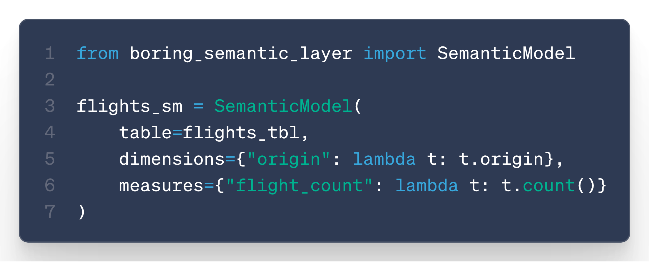
The first version of BSL kept things extremely straightforward:
One SemanticModel that takes as input:
1 Ibis table
measures, dimensions, and join definitions (defined as lambda functions)
Example:
Querying was just as simple as selecting dimensions and measures:
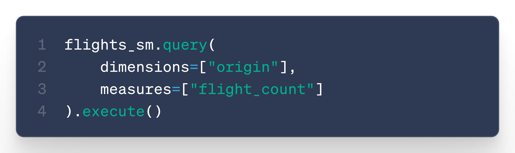
In that case, the output = a DataFrame with flight counts per origin.
We then extended around this concept with:
YAML support → define semantics in declarative files
Chart → query results as charts, not just DataFrames
MCP integration → expose the
query()method directly to LLMs
2- Limitations
As clean as v1 was, we hit a few walls quickly:
Complex aggregation
Things like percent of total, rankings, or rolling windows often require two steps:
Aggregate
Post-process
Our simple query()interface wasn’t expressive enough for these.
We considered adding a post_agg attribute, but that approach didn’t feel elegant or scalable.
Filters
In v1, filters were limited to dimensions:
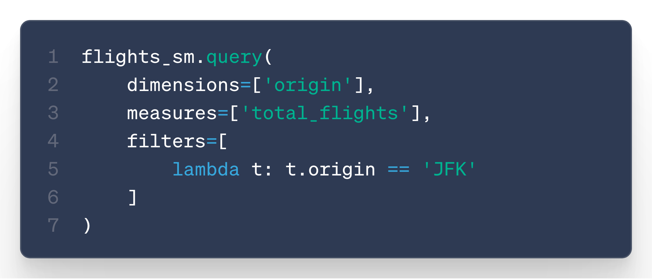
But users wanted more flexibility:
Filters before and after aggregation
Filters on dimensions, measures, or even raw table columns
Composability
In v1, the SemanticModel was the end of the road: once defined, you could only query it.
But in practice, teams want to compose models:
Marketing defines a Users semantic model
Support defines a SupportCases semantic model
Together, they want a metric: support cases per customer category
With v1, this meant rebuilding from raw tables again.
Not ideal.
Enter BSL v2
For BSL v2, we have decided to change its core and bring it to the next stage.
We’ve almost completely rewritten it, introducing a much deeper integration with Ibis.
To understand what changed in v2, it helps to take a step back and look at how Ibis itself works.
How Ibis works
At its core, Ibis doesn’t execute queries directly.
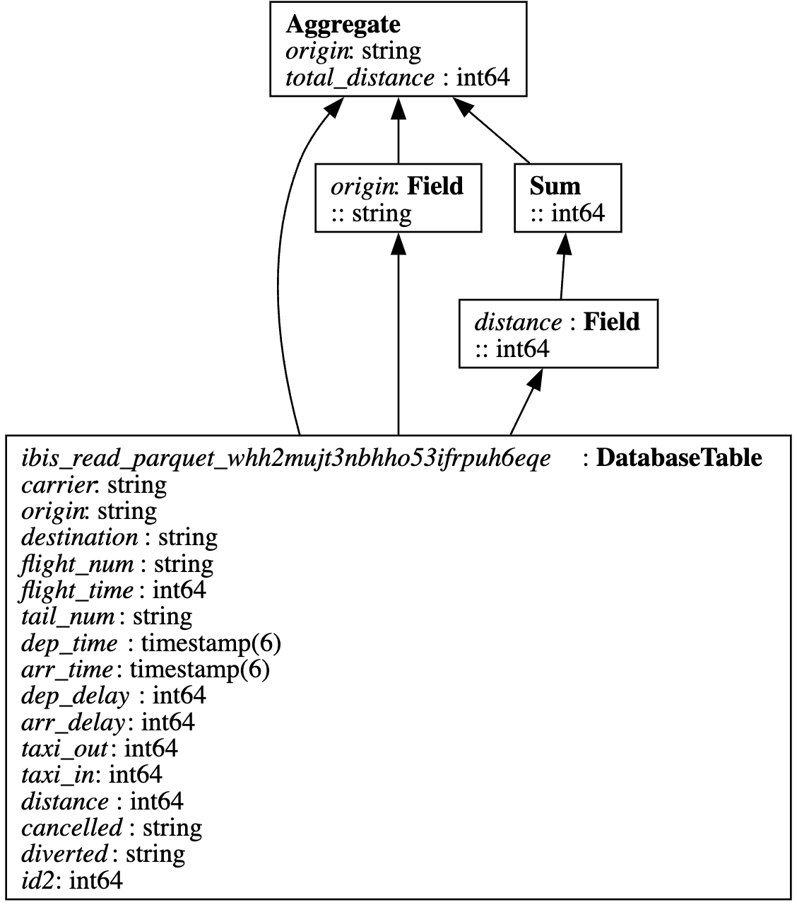
Instead, it builds an expression graph:
Every table, column, dimension, or measure you define is a node in the graph.
Each operation (like group_by, count, or filter) creates a new edge.
Let’s take the following ibis query:
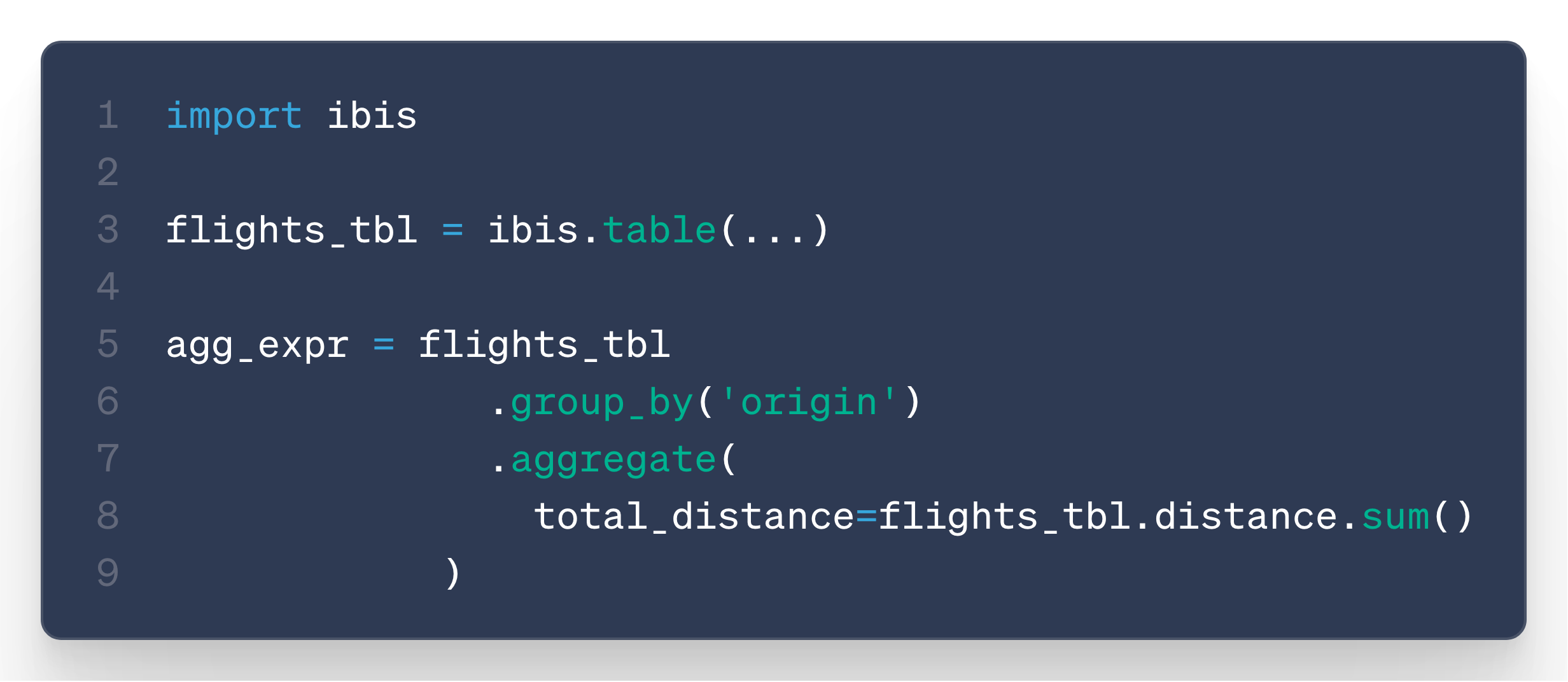
When the user defines agg_expr, no SQL is executed yet — Ibis creates the following expression graph:
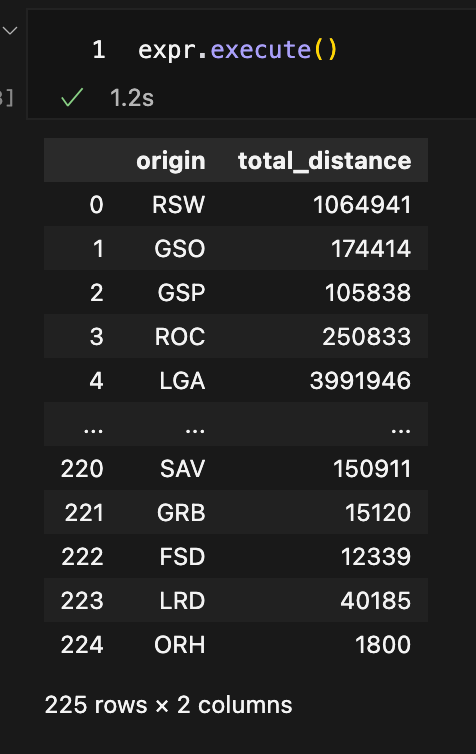
Only when you call .compile() or .execute() does Ibis translate the graph into the native SQL of your backend (DuckDB, BigQuery, Postgres, Snowflake, …):

In BSL v1, the semantic layer was essentially a query endpoint that sat on top of the Ibis graph without integrating into it.
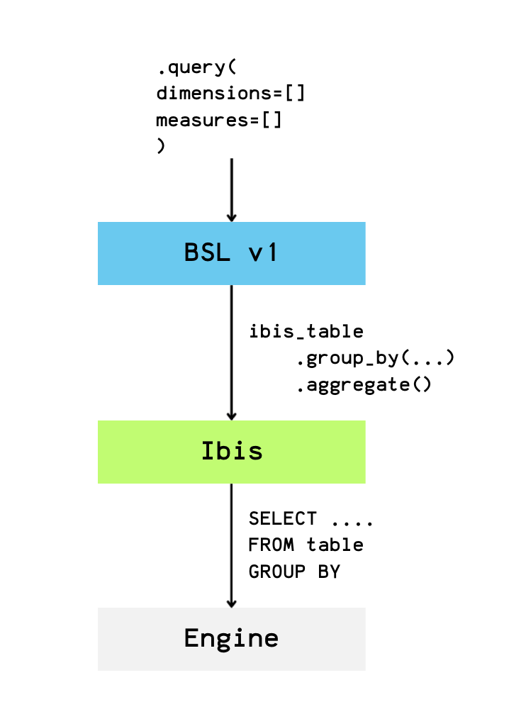
This means that dimensions and measures were not part of the expression graph itself, which limited composability and the ability to perform more complex transformations.
BSL is now part of the Ibis graph
With BSL v2, semantic models are now first-class nodes within the Ibis expression graph.
A semantic model is no longer just a query endpoint — it is a dedicated node in the graph that carries both dimension and measure metadata.
Concretely, this means we have introduced a new kind of Ibis table: semantic tables.
These are regular Ibis tables to which you can attach semantic information, such as definitions for dimensions and measures:
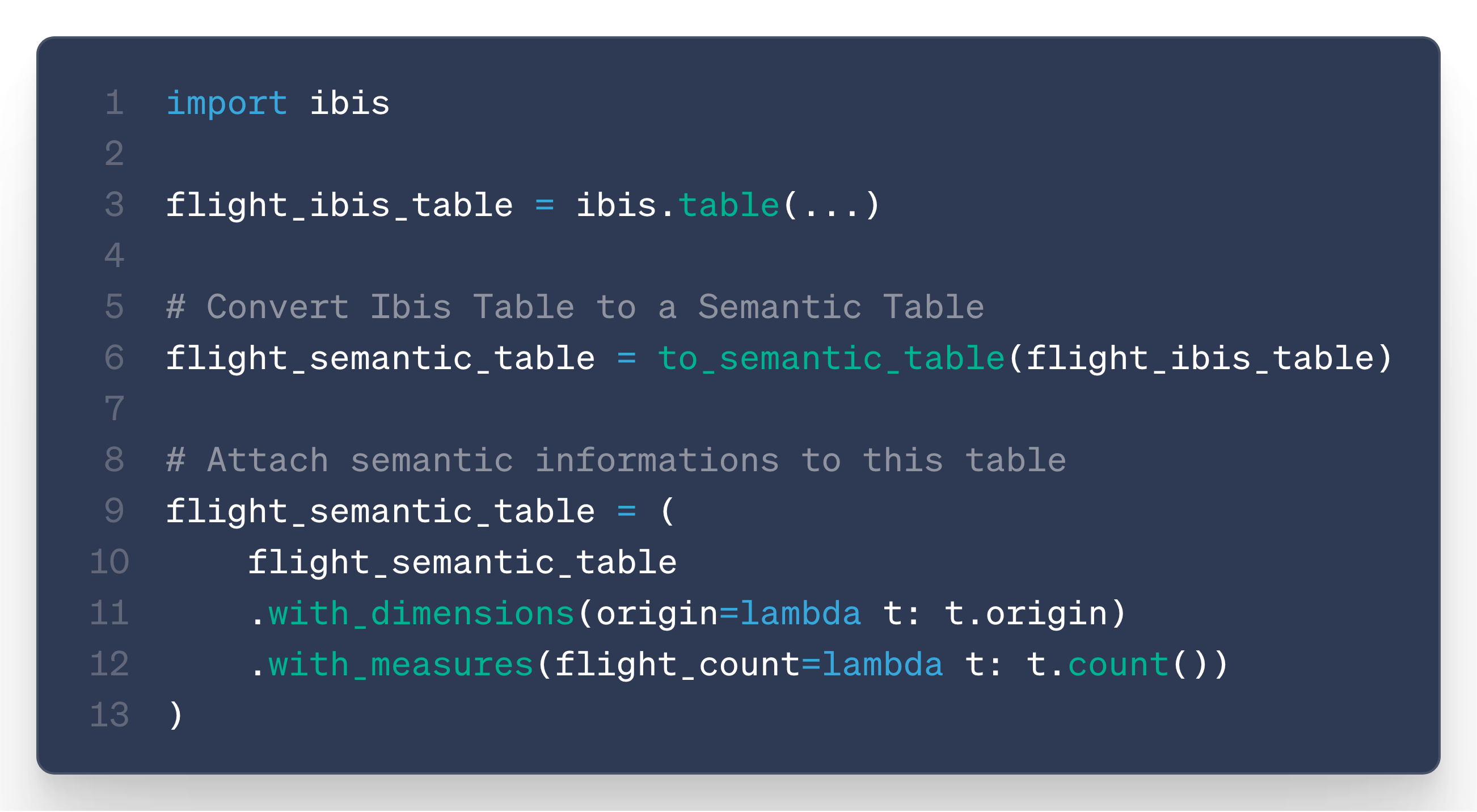
This table behaves like a regular Ibis table, but it also provides access to semantic metadata.
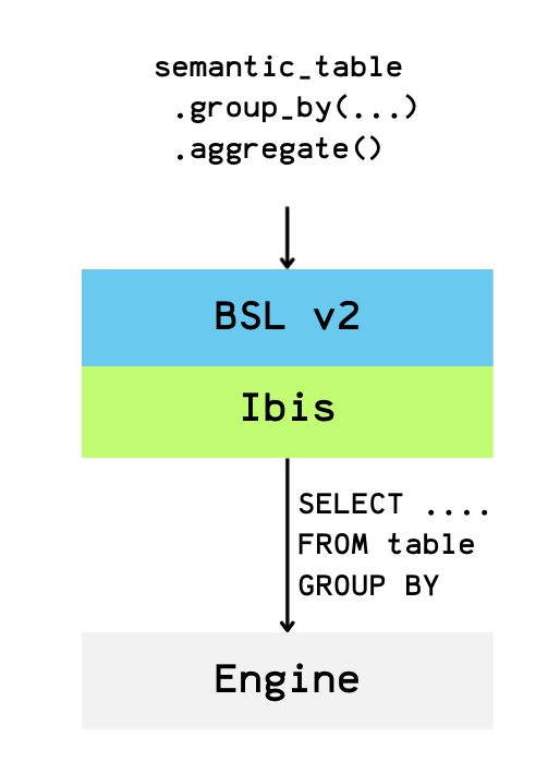
Want to select a dimension? → performs an ibis .group_by()
Want to select a measure? → performs an ibis .aggregate()
Querying your semantic model now feels like a regular Ibis query, but with a semantic layer:
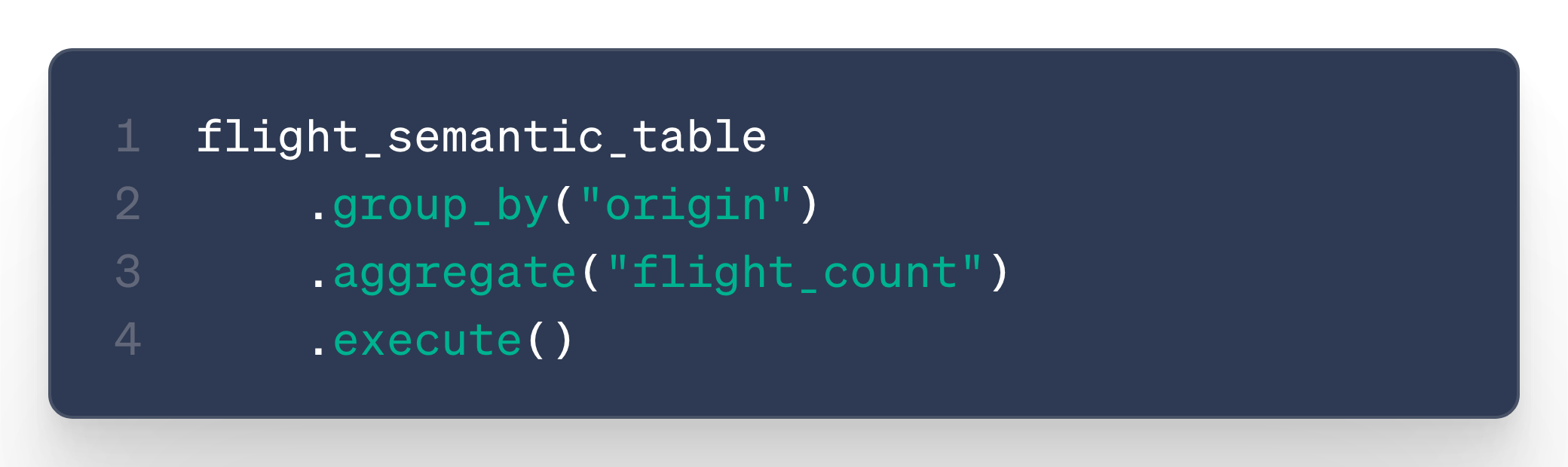
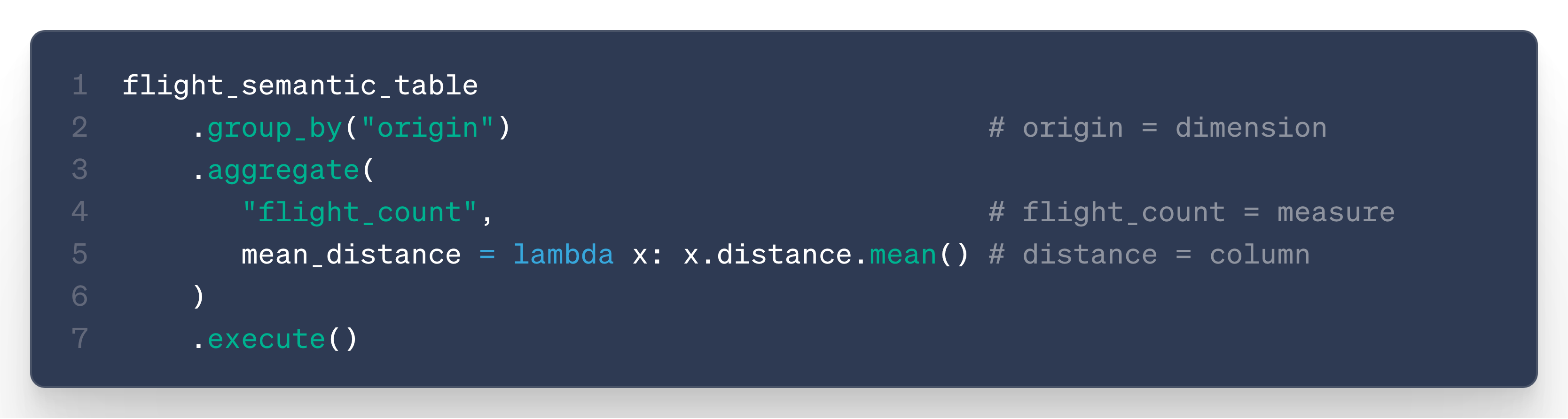
This makes queries highly flexible; users can also apply ad-hoc transformations directly on the semantic table:
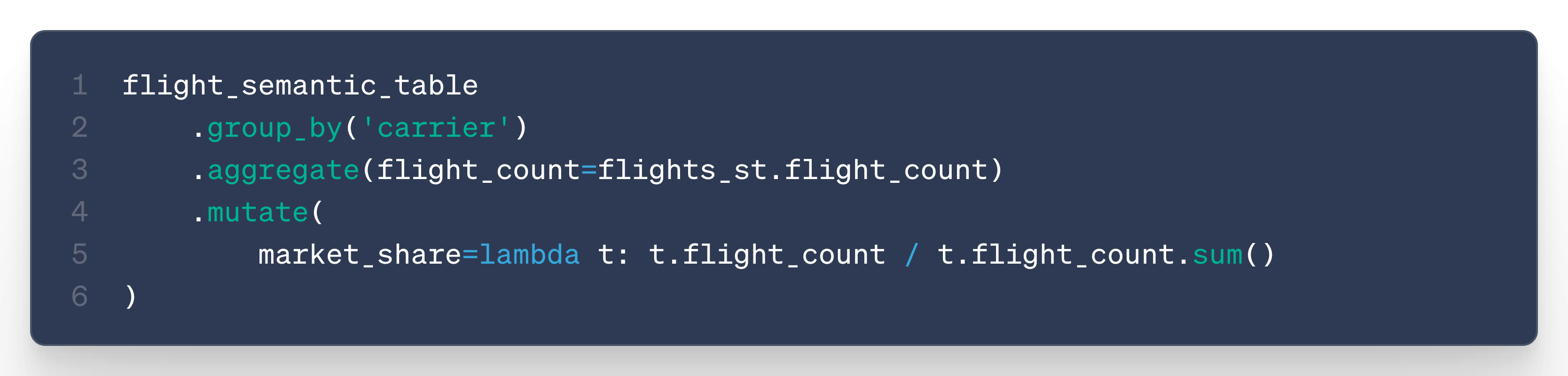
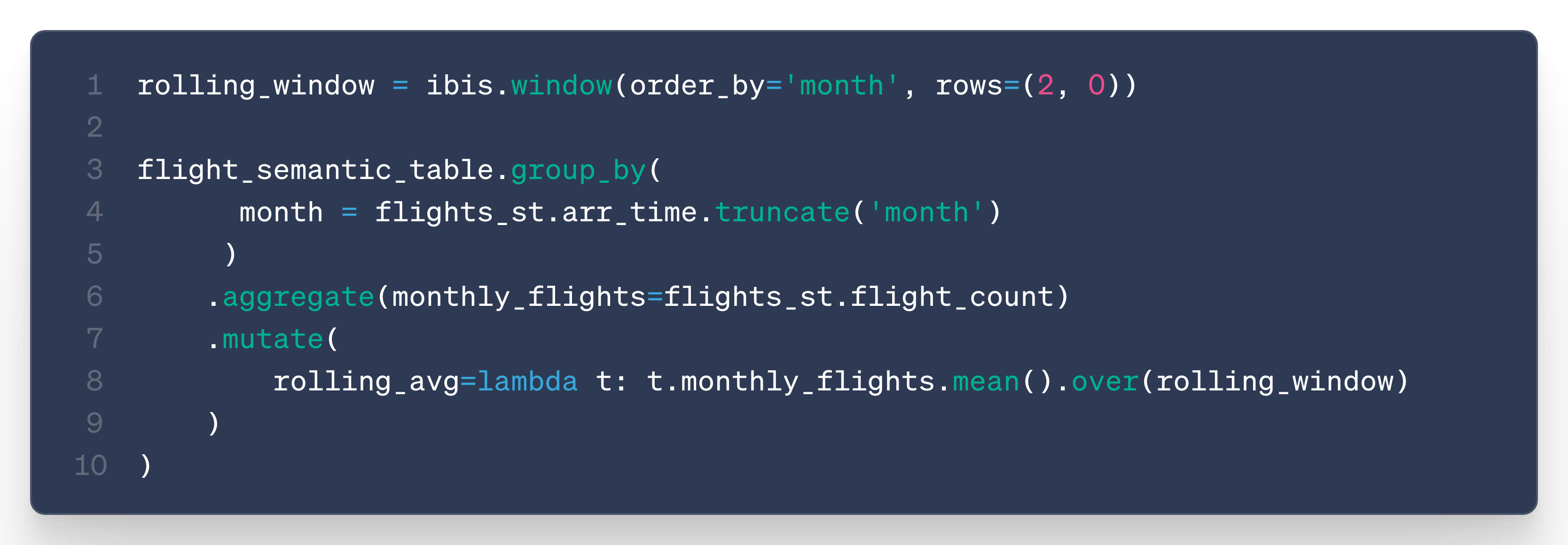
Additionally, this enables the use Ibis’s mutate() method, which allows post-aggregation and unlocks the following use cases:
Percentage of total:
Rolling averages
Composability
With v2, semantic tables are first-class nodes in the Ibis graph.
This means you can treat the output of one semantic table as the input to another, just like any other Ibis expression.
For example, imagine:
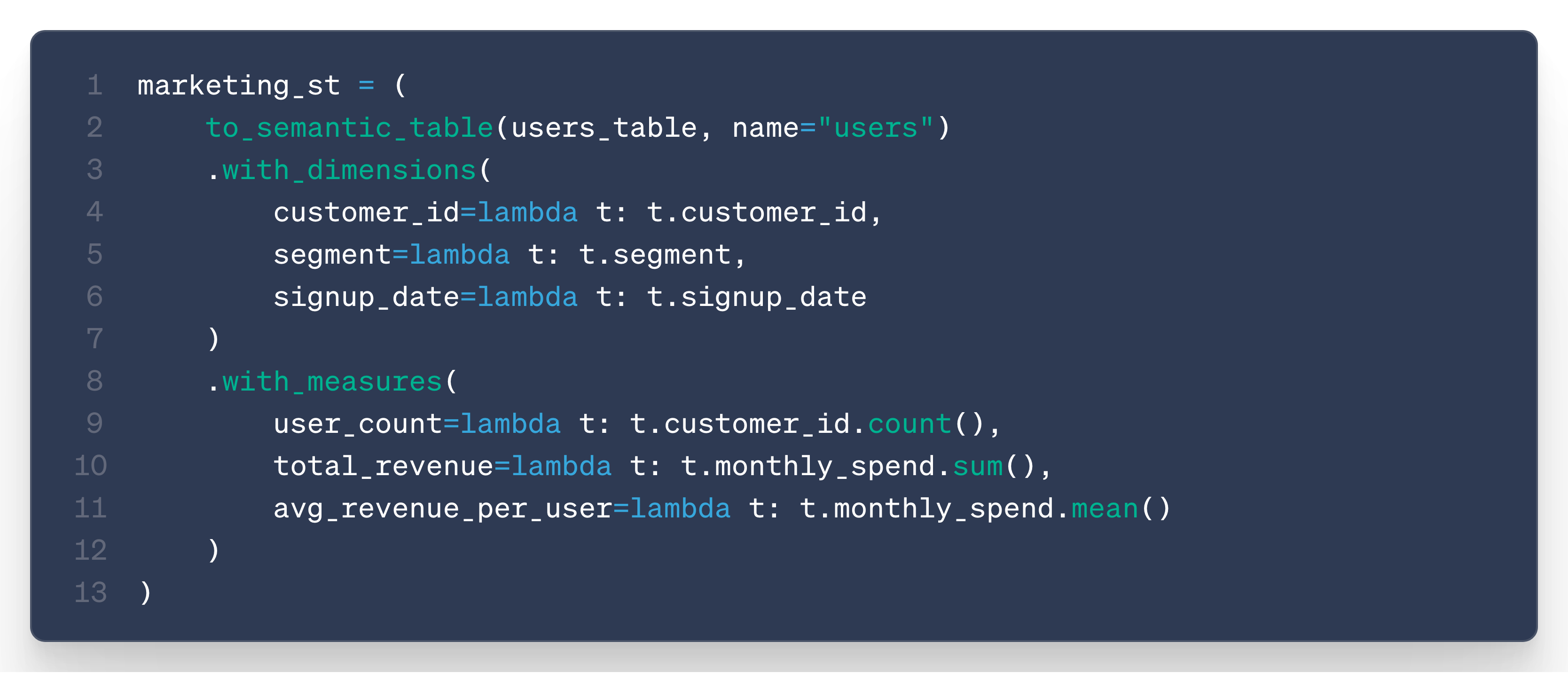
The marketing team defines a “User” semantic table.
The support team defines a “SupportCases” semantic table.
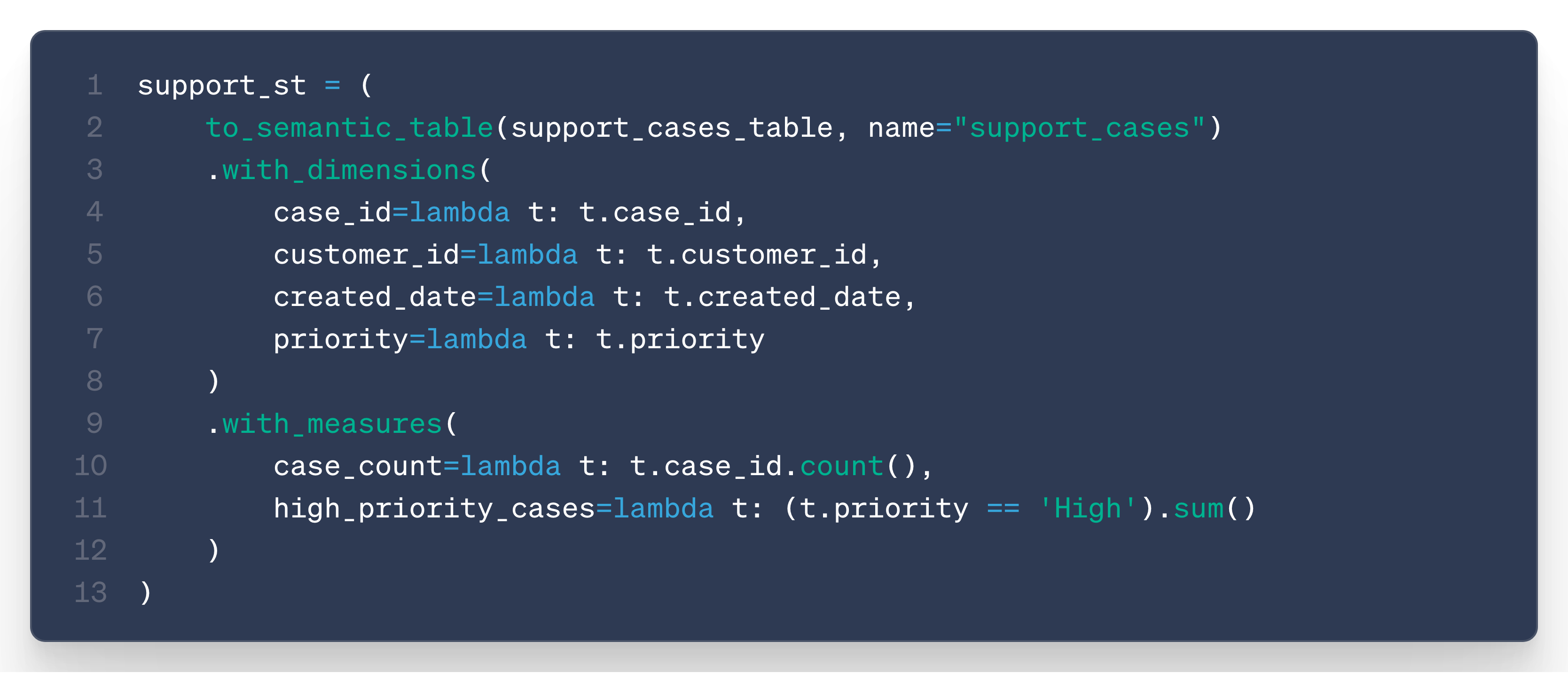
Together, they want a metric like support cases per customer segment, so they create a new semantic model built on top of these two existing models:
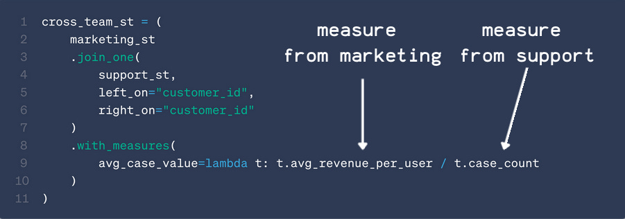
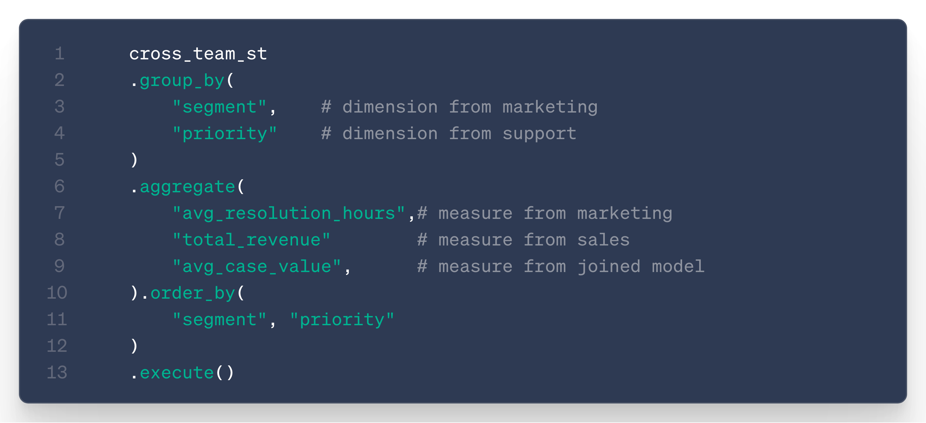
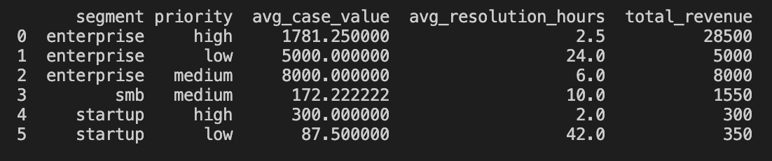
The user (or LLM) can then simply query the measure avg_case_value and aggregate it along any available dimension from any model.
All without worrying about where the underlying information comes from:
BSL v1→v2
Of course, all BSL v1 features remain fully compatible with v2:
YAML-based semantic definitions — you can still define semantic tables declaratively.
Charting — the .chart() method works as before, now directly on SemanticTable queries.
MCP integration — expose your semantic tables to LLMs via MCP just like in v1.
Next Step
One incredible advantage of BSL sharing the same API as Ibis is that LLMs are already fluent in Ibis :)
Additionally, LLMs can now execute their own Python code in a sandbox environment.
This means that with BSL, giving an LLM access to your semantic model is as easy as handing over a YAML file with your model definition.
No MCP, no server, no hosting, nada… just a boring YAML file.
But… that’s a topic for the next post :)
We are super excited by this new milestone for BSL.
We’re convinced that BSL is quickly becoming the lightest and most flexible semantic layer on the market.
A big thanks to all contributors who helped improve BSL over this summer.
If you share our enthusiasm:
Thanks for reading,
Hussain & Ju
 | A guest post by
|
Love this!